I’ve written before about both the gumbel-max trick and variational autoencoders. The world demanded a post that combined the two, so here it is. I mostly follow the repo for the DALL-E paper Ramesh et al. (2021). They also use the attrs package, which was nice to learn about, kinda neat, but a bit opaque.
As usual, I hope to entertain you with some of my mistakes and general troubles. If you are a sick, sick individual and came here to hear about taking the log of 0, I will happily indulge you. Here’s a Colab notebook if you’re on a similar learning journey and just need to see some code. Mega-disclaimer that I am just some dude, use at your own risk.
Categorical VAE’s
The general idea of categorical VAE’s is that our encoder learns the probabilities of a categorical distribution with \(K\) categories. These probabilities are used to sample from one of \(K\) vectors in a codebook (a collection of vectors). These sampled codebook vectors are then fed into a decoder to try to reconstruct the input.
Optimization is done in the usual way, by maximizing the evidence lower bound (ELBO, see my VAE post or other resources for details): \[ \begin{align} log(p(x)) \geq E_{z\sim q}[log(p(x \vert z;\theta))] - KL(q(z\vert x;\phi)\vert\vert p(z)) \end{align} \]
The first term on the RHS (the reconstruction objective) is usually defined as a Gaussian or Laplace distribution, and can be maximized with the \(l2\) or \(l1\) loss. In the paper, they use a different distribution called the logit-laplace distribution, with the reasoning that it models the distribution of pixel values better, specifically that they lie in a bounded range. The logit-laplace distribution is defined as:
\[ f(x, \mu, b) = \frac{1}{2bx(1-x)}\exp\left(-\frac{|logit(x) - \mu|}{b}\right) \]
They use the log of the RHS as the reconstruction objective, with the decoder outputting 6 channels per pixel location (3 \(\mu\)’s and 3 \(b\)’s for each pixel). I couldn’t tell you why this is better than assuming the inputs (between 0 and 1) are the probabilites of Bernoulli distributions, perhaps it is more flexible? But their concern of a bounded range is just as well taken care of by outputting values in the range \([0, 1]\) and using cross entopy with logits against the input image. In fact, I do this against MNIST (yes, its MNIST again, gimme a break ok).
The second (KL) term of the ELBO in the case of categorical VAE’s is comparing our encoder’s outputted distribution with a uniform categorical distribution over the \(K\) classes, which is easily calculated as:
\[ KL(q(z\vert x;\phi)\vert\vert p(z)) = \sum_{k=1}^K q(k\vert x;\phi) \log\left(\frac{q(k\vert x;\phi)}{1/K}\right) \]
since we assume \(p(z) = 1/K\) for all \(z\).
The Gumbel-(soft)Max Trick
Ok, if you remember in VAE’s we have to deal with this whole non-differentiable thing, since our process goes:
- Encode our input to the probabilities of a categorical distribution
- Sample from that distribution and use the sample to select a vector from a codebook.
- Decode the sample to try and match the input
and we cant backpropagate through 2. This is handled by using a relaxation of the Gumbel-max trick which if you’ll recall, is a way to sample from a categorical distribution by taking the arg-max of the log of the probabilities plus noise from a Gumbel(0,1) distribution. Arg-max isn’t differentiable, so we use softmax (which is more accurately described as soft-arg-max) as a differentiable approximation. We can adjust the temperature of the softmax operation to more closely approximate the arg-max operation.1
probs = self.encoder(x) # B x K x H x W
gumbel_noise = gumbel_sample(probs.shape).to(probs.device)

# apply softmax to log(probs) + gumbel noise divided by temperature tau.
# very small tau essentialy makes this one-hot
z = torch.nn.functional.softmax((probs.log() + gumbel_noise)/tau, dim=1)

# 'soft-samples' from the vector quantized embeddings
z = torch.einsum("bchw,cv -> bvhw", z, self.embedding)

# reconstruct to B x C x H x W
x_reconstr = self.decoder(z)
Notice that the probabilities are a B x vocab_size x H x W feature map. So we are sampling a vector from the codebook at each location in this feature map, or rather we are approximating sampling from it by taking a weighted (where the weights sum to one) combination of the codebook vectors, where one weight is very large is the rest are very small (due to the softmax operation). Once we have the reconstructed image and the probabilities of the categorical distribution, we can calculate the reconstruction loss and the KL divergence. The reconstruction loss is just:
reconstr_loss = nn.functional.binary_cross_entropy_with_logits(xrecon, x, reduction="mean")Or it would be the logit-laplace loss if I had implemented that:
def laplace_loss(x, mu, b):
    loss = -torch.log(2*b*x*(1-x)) - torch.abs(torch.logit(x) - mu)/b

    return loss
The KL divergence is as defined above, and can be calculated like so:
def KL_loss(logits, vocab_size=4096):
  loss = logits * (logits.log() - torch.log(torch.ones_like(logits)/vocab_size))

  # B x C x H x W
  return loss
…well, really I should be summing over the channel axis (KL definition has a sum), I do it in the notebook outside the function. As we’ll see later though, whether you sum or average is kinda arbitrary, because it seems empirical results suggests multiplying the KL loss by some constant is a good idea.
Mistakes were made
1) My first attempt was on the STL-10 dataset, which I leave code for in the notebook, but I couldn’t get the model to output good reconstructions. An example of one of the reconstructions:
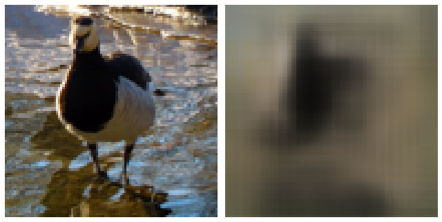
2) In the paper, they describe dividing the pixel values by 255, when performing preprocessing steps necessary to prevent divide-by-zeros in the logit-Laplace loss, which I gladly replicated without checking if my images were already 0-1 normalized. Funilly enough, it seemed to learn better than the non-normalized version, perhaps this is a clue to why I can’t get good quality samples from STL-10.
3) I had switched to cross-entropy loss, and was doing okay, until I got divide-by-zero errors. You see, I am calling softmax twice, once to do the Gumbel-softmax sampling, but also once before, in the encoder, to form the probabilities that go into the gumbel-softmax sampling. Remember we take the log of those values and then add Gumbel noise, so they all better be positive. Well, you might think that the softmax equation:
\[ softmax(z_i) = \frac{e^{z_i}}{\sum_{j=1}^n e^{z_j}} \]
would always produce positive values, but there’s this thing called numerical underflow which is a real pain in the ass, the ass of Daniel Claborne trying to take the logarithm of things, that is. Well, I just add a small constant and divide by the appropriate constant to make them still sum to 1 along the channel axis:
# forward method of the encoder
def forward(self, x):
    x = self.blocks(x)
    x = torch.nn.functional.softmax(x, dim = 1)

    x = (x + 1e-6)/(1 + self.vocab_size*1e-6)

    return x
4) I underestimated how much I would need to increase the importance of the KL term. In the paper, they multiply the KL loss term by \(\beta\) which is increased from 0 to 6.6 over some number of iteration. My initial attempts that stopped at \(\beta = 2\) produced poor sample quality, so I just tried their suggested \(\beta\)
Some success with MNIST
Ok, I was defeated by STL-10 (I’ll try again once Colab gives me some more compute credits), but good ol easy-mode MNIST gave me some nice results. I load my best test loss model from https://wandb.ai/clabornd/VQVAE/runs/9bb6w3ru?workspace=user-clabornd and use it to generate some samples.s
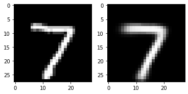
First, we see if it can reconstruct an image that is passed to the encoder. Intuitively the encoder should map the image \(X\) to a latent representation \(z\) that is likely to produce something similar to \(X\) in the output, and so it does as seen in Figure 2.
But remember we not only wanted to be able to produce an image when providing an image, but be able to produce images when sampling from random noise. This is the point of the KL loss term, making the latent representation close to a uniform categorical distribution. We should then be able to sample from a uniform categorical (for each pixel location in a latent feature map), pass this sample to our decoder, and get things that look like our training data. And so we do (sorta):
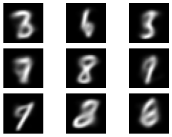
Wow, what a bunch o beauts’. Hopefully I can get you some pictures of slightly less blurry birds/airplanes soon.
References
Footnotes
In the paper they start with temperature \(tau = 1\) and reduce it to \(\frac{1}{16}\) over some number of iterations - I do as well in the notebook.↩︎