Vectorize Your Sampling from a Categorical Distribution Using Gumbel-max! Use pandas.DataFrame.shift() more!
Behind this disaster of a title lies the secret to quickly sample from a categorical distribution in python!
data science
code
Author
Daniel Claborne
Published
November 28, 2022
Honestly, what a disaster of a title. I don’t know if either part in isolation would be more likely to get someone to read this, but I just wanted to make a post. Maybe I should have click-baited with something completely unrelated, oh well.
I’m currently taking Machine Learning for Trading from the Georgia Tech online CS masters program as part of my plan to motivate myself to self-study by paying them money. While much of the ML parts of the class are review for me, it has been fun to learn things about trading, as well as do some numpy/pandas exercises.\(^{[1]}\)
The class is heavy on vectorizing your code so its fast (speed is money in trading), as well working with time series. I’ll go over two things I’ve found neat/useful. One is vectorizing sampling from a categorical distribution where the rows are logits. The other is using the .shift() method of pandas DataFrames and Series.
Vectorized sampling from a categorical distribution
Okay, so the setup is you have an array that looks like this:
import numpy as npnp.random.seed(23496)# The ML people got to me and I now call everything that gets squashed to a probability distribution 'logits'logits = np.random.uniform(size = (1000, 10))logits = logits/logits.sum(axis =1)[:,None]logits[:5,:]
Each row can be seen as the bin probabilities of a categorical distribution. Now suppose we want to sample from each of those distributions. One way you might do it is by leveraging apply_along_axis:
Hm, okay this works, but it is basically running a for loop over the rows of the array. Generally, apply_along_axis is not what you want to be doing if speed is a concern.
So how do we vectorize this? The answer I provide here takes advantage of the Gumbel-max trick for sampling from a categorical distribution. Essentially, given probabilities \(\pi_i, i \in {0,1,...,K}, \sum_i \pi_i = 1\) if you add Gumbel distribution noise to the log of the probabilites and then take the max, it is equivalent to sampling from a categorical distribution.
Again, take the log of the probabilities, add Gumbel noise, then take the arg-max of the result.
16 ms ± 200 μs per loop (mean ± std. dev. of 7 runs, 100 loops each)
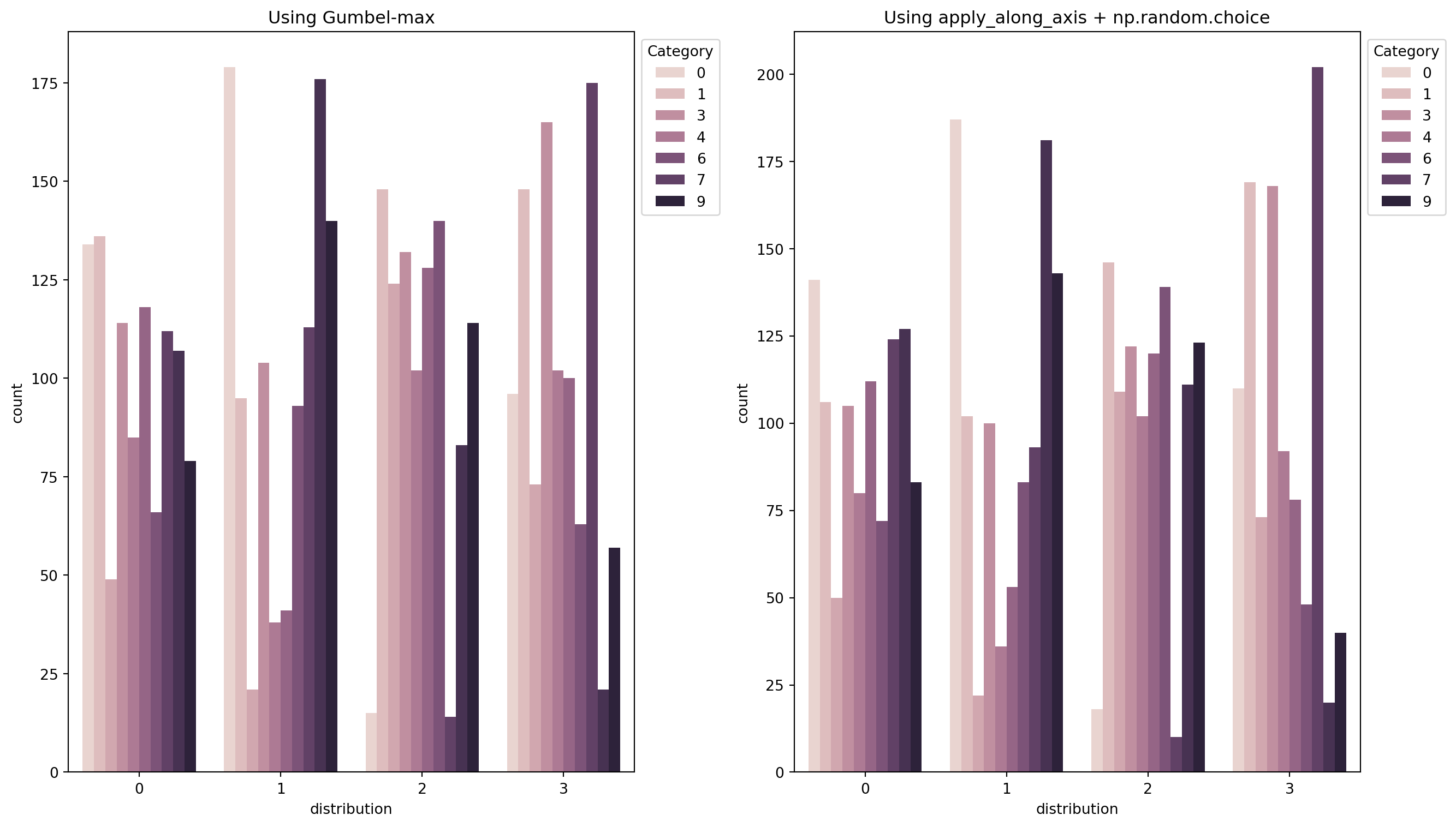
Yea, so a couple orders of magnitude faster with vectorization. We should probably also check that it produces a similar distribution across many samples (and also put a plot in here to break up the wall of text). I’ll verify by doing barplots for the distribution of 1000 values drawn from 4 of the probability distributions. Brb, going down the stackoverflow wormhole because no one knows how to make plots, no one.
…
Ok I’m back, here is a way to make grouped barplots with seaborn:
import matplotlib.pyplot as pltimport seaborn as snsimport pandas as pd# do 1000 draws from all distributions using gumbel-maxgumbel_draws = []for i inrange(1000): samples = ( np.log(logits) + np.random.gumbel(size = logits.shape) ).argmax(axis =1) gumbel_draws.append(samples) gumbel_arr = np.array(gumbel_draws)# ...and 1000 using apply_along_axis + np.random.choiceapply_func_draws = []for i inrange(1000): samples = np.apply_along_axis(lambda x: np.random.choice(range(len(x)), p=x), 1, logits ) apply_func_draws.append(samples)apply_func_arr = np.array(apply_func_draws)
In the above, if you ran the two for loops separately, you would get a better sense of how much faster the vectorized code is. Now well munge these arrays into dataframes, pivot, and feed them to seaborn.
The distribution of drawn values should be roughly the same.
Eyeballing these, they look similar enough that I feel confident I’ve not messed up somewhere.
Finally, of note is that a modification of this trick is used a lot in training deep learning models that want to sample from a categorical distribution (Wav2vec(Baevski et al. 2020) and Dall-E(Ramesh et al. 2021) use this). I’ll go over it in another post, but tl;dr, the network learns the probabilities and max is changed to softmax to allow backpropagation.
pandas.DataFrame.shift()
You could probably just go read the docs on this function, but I’ll try to explain why its useful. We often had to compute lagged differences or ratios for trading data indexed by date. To start I’ll give some solutions that don’t work or are bad for some reason, but might seem like reasonable starts. Lets make our dataframe with a date index to play around with:
import pandas as pdmydf = pd.DataFrame( {"col1":np.random.uniform(size=100), "col2":np.random.uniform(size=100)}, index = pd.date_range(start ="11/29/2022", periods=100))mydf.head()
col1
col2
2022-11-29
0.291912
0.865337
2022-11-30
0.846767
0.566933
2022-12-01
0.922189
0.317249
2022-12-02
0.348480
0.865872
2022-12-03
0.527629
0.658990
Now, suppose we want to compute the lag 1 difference. Specifically, make a new series \(s\) where \(s[t] = col1[t] - col2[t-1]: t > 0\), \(s[0] =\) NaN. Naive first attempt:
Uh, so what happened here? Well, pandas does subtraction by index, like a join, so we just subtracted the values at the same dates, but the first and last dates were missing from col1 and col2 respectively, so we get NaN at those dates. Clearly this is not what we want.
Another option converts to numpy, this is essentially just a way to move to element-wise addition:
Ok, its the same length and has the right values so we can put it back in the dataframe as a column or create a new series (and add the index again)
# make a new serieslag1_series = pd.Series(lag1_arr, index=mydf.index)# or make a new column# mydf["col3"] = lag1_arr
Alright, but this looks kinda ugly, we can do the same thing much more cleanly with the .shift() method of pandas DataFrames and Series. .shift(N) does what it sounds like, it shifts the values N places forward (or backward for negative values), but keeps the indices of the series/dataframe fixed.
mydf["col1"].shift(3)
2022-11-29         NaN
2022-11-30         NaN
2022-12-01         NaN
2022-12-02    0.291912
2022-12-03    0.846767
                ...
2023-03-04    0.053952
2023-03-05    0.816689
2023-03-06    0.540073
2023-03-07    0.202409
2023-03-08    0.409475
Freq: D, Name: col1, Length: 100, dtype: float64
With this we can easily compute the lag 1 difference, keeping the indices and such.
# differencemydf["col1"] - mydf["col2"].shift(1)# lag 3 ratiomydf["col1"]/mydf["col2"].shift(3)
2022-11-29         NaN
2022-11-30         NaN
2022-12-01         NaN
2022-12-02    0.402710
2022-12-03    0.930673
                ...
2023-03-04    0.203755
2023-03-05    0.465254
2023-03-06    0.048714
2023-03-07    0.534919
2023-03-08    0.751147
Freq: D, Length: 100, dtype: float64
This lag-N difference or ratio is extremely common and honestly I can’t believe I hadn’t been using .shift() more.
\(^{[1]}\)I am not affiliated with GA-Tech beyond the new washing machine and jacuzzi they gave me to advertise their OMSCS program
References
Baevski, Alexei, Henry Zhou, Abdelrahman Mohamed, and Michael Auli. 2020. “Wav2vec 2.0: AFramework for Self-SupervisedLearning of SpeechRepresentations.”arXiv:2006.11477 [Cs, Eess], October. http://arxiv.org/abs/2006.11477.
Ramesh, Aditya, Mikhail Pavlov, Gabriel Goh, Scott Gray, Chelsea Voss, Alec Radford, Mark Chen, and Ilya Sutskever. 2021. “Zero-ShotText-to-ImageGeneration.” arXiv. https://doi.org/10.48550/arXiv.2102.12092.